Transcriptomics II
- Methods of Exploratory Data Analysis
- Clustering
- Dimensionality Reduction
- Differential Expression Analysis
Methods of Exploratory Data Analysis
Typical shape of data we have in hand: a data matrix.
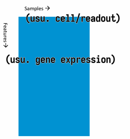
where the columns are the samples and the rows are the features (usually gene expressions). (It can be the other way around, but this is the most common case.)
- Clustering
- Hierarchical clustering
- k-means clustering
- Dimensionality reduction
- Matrix Factorization
- PCA
- MDS (Multidimensional Scaling)
- Graph-based methods
- t-SNE
- UMAP
- Matrix Factorization
Clustering
- Goals
- group similar samples
- evaluate similarity between expression profiles of the samples
- test if similarities match the experimental design and effect sizes
- test if variations within condition is smaller than between conditions
- outliers detection
- group similar genes
- guilt by association: infer functions of unknown genes from known genes with the same expression pattern (co-expression)
- group similar samples
Distance measures
To cluster samples, we need to first define a "distance" measure between samples.
Commonly used distance measures:
- Euclidean distance (typically for clustering samples)
- Euclidean distance of two profiles $\mathbf{x}$ and $\mathbf{y}$ with $p$ genes (i.e. the distance between two $p$-dimensional vectors $\mathbf{x}$ and $\mathbf{y}$)
- $d(\mathbf{x}, \mathbf{y}) = \sqrt{\sum_{i=1}^{p} \left(x_i - y_i\right)^2}$
- Expression values MUST BE LOG SCALE
- $1 - \text{corr}(\mathbf{x}, \mathbf{y})$ (typically for clustering genes)
- Correlation coefficient of two profiles $\mathbf{x}$ and $\mathbf{y}$ with $p$ samples
- $\text{corr}(\mathbf{x}, \mathbf{y}) = \frac{\sum_{i=1}^{p}(x_i - \bar{x})(y_i - \bar{y})}{\sqrt{\sum_{i=1}^{p}(x_i - \bar{x})^2 \cdot \sum_{i-1}^{p}(y_i - \bar{y})^2}}$
- $\bar{x} = \frac{1}{p}\sum_{i=1}^{p}x_i$
- $\bar{y} = \frac{1}{p}\sum_{i=1}^{p}y_i$
Hierarchical Clustering
Algorithm:
- Compute the distance matrix ($n \times (n - 1) / 2 \rightarrow O(n^2)$) between all samples
- Find pair with minimal distance and merge them
- Update the distance matrix
- Repeat 2-3 until all samples are merged
Parameters:
- distance measure for samples
- usually $1 - \text{corr}(\mathbf{x}, \mathbf{y})$ for gene expression
- distance measure for clusters (linkage rule)
- Single linkage: minimum distance between any elements of the two clusters
- Complete linkage: maximum distance between any elements of the two clusters
- Average linkage: average distance between all elements of the two clusters
- Ward's linkage: minimal increase in intra-cluster variance
Input:
- distance matrix
- The linkage can be derived directly from the distance matrix.
- Hence clustering algorithm only needs the distrance matrix as input, not the measurements individually.
k-means Clustering
Algorithm:
- Randomly assign each sample to one of the $k$ clusters
- Compute the centroid (cluster center, average of the assigned samples) of each cluster
- Assign each sample to the cluster with the closest centroid
- Repeat 2-3 until convergence or a maximum number of iterations
Parameters:
- number of clusters $k$
- distance measure for samples
Input:
- data matrix (cannot directly use distance matrix)
This method minimizes the intra-cluster variance.
Choice of $k$ affects the result.
Comparison of Hierarchical Clustering and k-means Clustering
| Hierarchical Clustering | k-means Clustering | |
|---|---|---|
| Computing time | $O(n^2 \log (n))$ | $O(n \cdot k \cdot t)$
|
| Memory | $O(n^2)$ | $O(n \cdot k)$ |
When clustering large numbers of genes (>1e4, hierarchical clustering is not practical
Dimensionality Reduction
Principal Component Analysis (PCA)
Goal: Find a new coordinate system such that the first axis (principal component) captures the most variance, the second axis captures the second most variance, and so on.
The data is linearly transformed to a new coordinate system.
t-SNE
Algorithm:
- In the high-dimensional space, create a probability distribution that dictates how likely two points are to be neighbors.
- Recreate a low dimensional space that follows the same probability distribution as best as possible.
How to find the best low-dimensional representation:
- preserve the pairwise distances between neighboring points in the high-dimensional space
- non-linear, different transformations on different regions
Characteristic:
- Powerful, but need to fiddle with random seed and perplexity
- Non-deterministic
UMAP
Uniform Manifold Approximation and Projection
Approach: Find for each point the neighbors and build simplices (simplex: a generalization of the concept of a triangle or tetrahedron to arbitrary dimensions) and then optimize the low-dimensional representation to preserve the simplices.